Why This Project?
Hurricanes are chaotic. The atmosphere doesn't play nice with predictions, observational data over oceans is sparse, and forecasters need answers fast. Traditional numerical weather models demand supercomputer-level resources and still miss short-term movements.
I wanted to see if a lightweight CNN could do better—specifically, predict where a storm will be 6 hours from now using freely available reanalysis data.
The Data Problem
Two data sources power this system:
- ERA5 Reanalysis — Gridded atmospheric fields from ECMWF, downloaded as monthly NetCDF files via the CDS API. I built an LRU-style cache to avoid hammering the disk.
- HURDAT2 Best Tracks — Ground-truth storm positions at 6-hour intervals, stored as JSON indexed by timestamp.
The tricky part? ERA5 uses 0–360° longitude. HURDAT uses -180/180°. Storms cross the date line. I spent more time than I'd like to admit wrestling with xr.roll() and coordinate reassignment to make these play together.
What Goes Into the Model
For each timestep, I extract a 70° × 70° box centered on the storm, then resize it to a clean 40 × 40 × 17 tensor:
- 5 surface channels: 10m winds (u, v), sea level pressure, SST, water vapor
- 12 pressure-level channels: Wind components + relative humidity at 200, 500, 700, and 850 hPa
The target is dead simple: next_position - current_position. Just the displacement in degrees.
The CNN Architecture
I optimized for parameter efficiency without sacrificing spatial awareness:
- Separable Convolutions — Fewer parameters, same spatial feature extraction
- Residual Block — 1×1 shortcut + dual separable convs. Helps when atmospheric patterns are persistent (the model can learn "just pass it through")
- Channel Attention — The model learns which variables matter most. Sometimes SST dominates; sometimes it's wind shear
- Spatial Attention — Hurricanes aren't symmetric. This lets the model focus on the relevant quadrant
The head is straightforward: GlobalAveragePooling → Dense(128) → Dense(64) → Dense(2) outputting [Δlat, Δlon].
Running Inference
At prediction time:
- Load saved normalization stats
- Build the feature tensor for the current timestep
- Forward pass → denormalize the output
- Add the predicted delta to current position
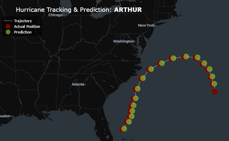
Error is measured via Haversine approximation (roughly Δ° × 111 km). Visualization uses Plotly Scattermaps—actual tracks overlaid with predictions, bubble size scaled to storm radius, color-coded by intensity.
The Baseline: SHIPS + XGBoost
Not everything needs a CNN. I also built a tabular baseline using SHIPS diagnostic files—10 scalar features (lat, lon, vmax, pressure, SST, ocean heat content, shear, humidity, distance to land, MPI) fed into XGBoost for 24-hour predictions.
It's faster, needs no GPU, and provides a sanity check. The CNN wins on accuracy, but the gap isn't as large as you might expect.
Edge Cases I Had to Handle
- Zero-dimension tensors — TensorFlow crashes hard if you don't validate shapes before resize
- Storm ID mismatches — Had to filter to ensure consecutive timesteps belong to the same system
- Memory leaks — ERA5 cache gets cleared after each storm to prevent file handle exhaustion
- Coordinate hell — Longitude sign conventions differ between every data source. Fixed in slicing and rendering